Why INLA-SPDE Changes Plume Estimation

Remediation cost is tightly coupled to the volume of contaminated soil. A representative site at 3,822 m³ costs between $290,000 and $879,000 to remediate at typical Canadian unit rates of $76 to $230 per m³ [1]. Underestimate the plume and the contractor returns six months later to re-excavate, paying mobilisation a second time. Overestimate it and the project trucks out clean soil at the same rate as contaminated soil. The financial leverage is brutal, and most of the leverage is decided before the first scoop of dirt moves, when a statistical model converts a handful of borehole logs into a three-dimensional estimate of where contamination lives.

The standard tool for that conversion is Kriging, and Kriging was not designed for the data we actually collect. Most contaminated sites yield small, zero-inflated datasets from boreholes placed where the plume is suspected to be, not where statistical theory says they should be. Soil structure at brownfield and post-remediation sites is fractured and irregular from prior drilling, excavation, and treatment work. Preferential flow runs through that disturbed matrix in pathways that the geostatistical assumption of a smooth, predictable gradient never sees. The result is the cost overrun that practitioners now treat as a normal part of the work.

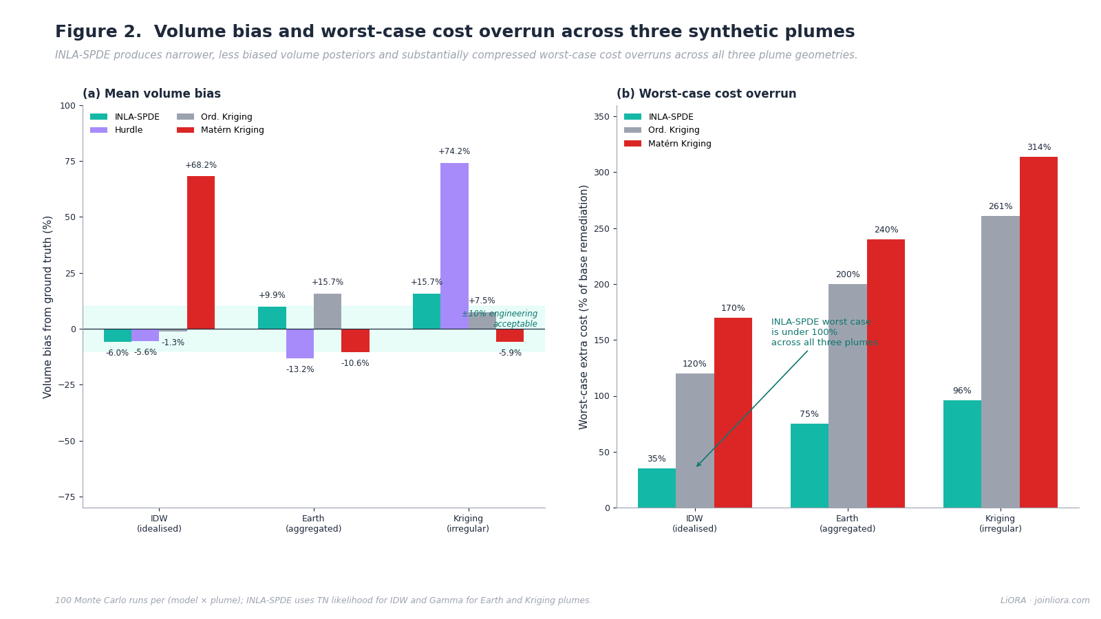
Our group has been working on a different foundation. In a recent manuscript, we adapted the Integrated Nested Laplace Approximation with a Stochastic Partial Differential Equation, or INLA-SPDE, to plume estimation at petroleum hydrocarbon sites [2]. Across three synthetic plumes with known geometry and two real bioremediation sites, INLA-SPDE produced stable, defensible plume volume and mass estimates with as few as five boreholes. The expected-cost overrun against ground truth shrank to 17 to 37 percent of the base remediation cost, compared with 24 to 106 percent for Kriging-based methods. The worst-case scenario, the one that determines whether a project goes over its bond, compressed from 261 to 314 percent under Matérn Kriging down to 35 to 96 percent under INLA-SPDE. The improvement is large enough that the technique changes what kinds of sites can be characterised defensibly within a given borehole budget.

This piece walks the technical foundation, the numbers from the synthetic and real-site evaluation, and the cost arithmetic, and then closes on why this work matters for what we call Digital Shadowing of environmental behaviour. The short version is that Digital Shadowing is only as good as the spatial mathematics underneath it, and INLA-SPDE is the first framework we have tested that meets the requirements of zero-inflated, sparse, irregularly sampled contaminant data without breaking.

Why Plume Estimation Is a Statistically Hard Problem

Soil contaminant datasets violate the assumptions of classical geostatistics in four ways that practitioners encounter every week.

Sparse sampling. Borehole counts at contaminated sites are constrained by budget, accessibility, and the schedule pressure of remediation. Five to twelve boreholes for a residential or commercial site is common. The Kriging variogram needs more data than that to be fit reliably, and the geostatistical literature has long acknowledged that small sample sizes inflate Kriging uncertainty in ways that propagate forward into volume estimates [3]. When a site has eight boreholes, the variogram is being conditioned on tens of pairwise distances, and the spherical fit is doing more work than the data warrants.

Zero-inflation. Improved analytical technology pushes detection limits lower, and lower detection limits produce datasets where a large fraction of measurements come back at or near zero. In our two field sites, the share of values below the 0.0001 mg kg⁻¹ detection limit for benzene exceeded fifty percent for several sample sets. Zero-Inflated Poisson and Zero-Inflated Negative Binomial models address inflated zeros for count data, but contaminant concentrations are continuous, right-skewed, and censored, not counted. The Hurdle structure, which models the probability of exceeding the detection limit and the magnitude of exceedance separately, is the right shape, but it needs to be combined with a continuous likelihood that can absorb the censoring.

Preferential flow. In disturbed soil, contaminants do not migrate uniformly. They move through fracture networks, backfill seams, utility trenches, and the relict structure left by prior excavations. The lateral and vertical distribution that results is not a smooth surface centred on a hotspot. It is patchy, anisotropic, and often discontinuous. A model that does not have a way to ingest information about flow paths cannot represent this geometry, and the residuals it produces will look like noise even when the underlying process is highly structured.

Disturbed soil structure. The places where plume estimation matters most, brownfield redevelopment, post-remediation closeout, and Phase II assessment at legacy sites, are also the places where the subsoil has been most thoroughly rearranged. The Kriging assumption of a smooth, predictable spatial gradient centred around hotspots is built for sites that have not been touched. At a site with a history of underground storage tank removal, soil excavation, and biostimulation injection, the assumption is wrong before the variogram is fit.

Preferential borehole placement. Boreholes at contaminated sites are intentionally located where contamination is considered most likely based on site history, field observations, and risk assessment. This targeted strategy is highly effective for contaminant detection and regulatory decision-making, but it does not necessarily provide the spatial coverage needed for reliable plume estimation. In particular, boreholes are often concentrated around suspected hotspots while few are placed near plume boundaries or in apparently clean areas. Under these conditions, Kriging must infer plume extent from limited boundary information, making contaminant volume and mass estimates highly sensitive to variogram assumptions. The challenge is therefore not sparse sampling, but a mismatch between a risk-driven sampling design and the statistical requirements of spatial interpolation.

The combined effect is a statistical environment where the workhorse tool is being asked to do work it was never built for. Some of the cost overruns that show up in remediation post-mortems trace back to this mismatch, not to operational execution.

The INLA-SPDE Framework

The INLA-SPDE approach replaces four pieces of the standard Kriging workflow at once. None of the pieces is novel on its own. The combination, applied to contaminant plume estimation, is.

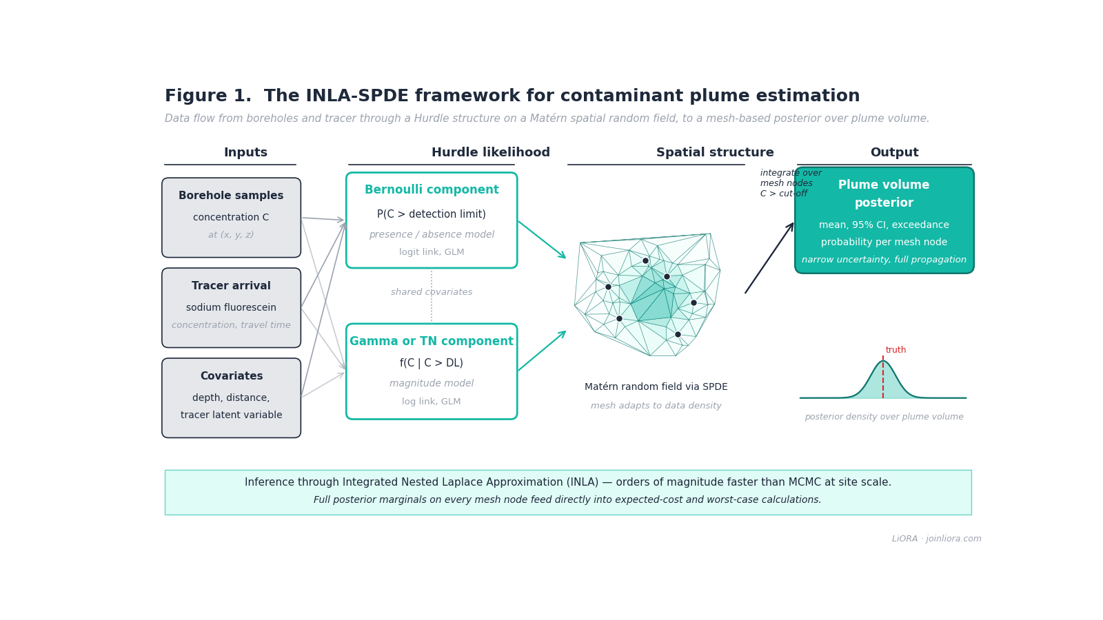
A Hurdle Structure for Zero-Inflated Data

We model concentrations in two stages. A Bernoulli likelihood estimates the probability that the concentration at a given location exceeds the detection limit. Conditional on exceedance, a second likelihood models the magnitude. We tested two choices for that second likelihood. A truncated normal worked best for moderately skewed datasets like the Inverse Distance Weighted (IDW) synthetic plume. A Gamma likelihood performed better for the heavily left-censored, strongly skewed real-site datasets and for synthetic plumes generated with Earth and Kriging interpolation. The combined hurdle structure looks like this:

P(C_i = 0 | X_i) = 1 - π_i
P(C_i > 0 | X_i) = π_i · f(C_i; θ_i)


where π_i is the modelled probability of exceeding the detection limit, and f is either a truncated normal density with mean and variance estimated from the data, or a Gamma density with shape and rate parameters estimated from the data. Both components share the same set of covariates, which keeps the model tractable and allows the same physical drivers to inform both the presence and the magnitude of contamination.

Mesh-Based Geometry Instead of Fixed Grids

Conventional Kriging discretises space onto a user-defined grid before computing volumes. The grid spacing is a modelling decision that bleeds into the answer. Coarse grids smooth over the plume edge; fine grids spike the computational cost and over-resolve the underlying data.

INLA-SPDE uses a triangulated mesh whose vertex density adapts to the spatial distribution of the boreholes [4]. Each mesh node owns a representative volume defined by the local triangulation, and the plume volume is the sum of those node-volumes where the predicted concentration exceeds the regulatory cut-off. The mesh is constructed once from the borehole geometry and used for both inference and integration, which removes a degree of analyst discretion from the volume estimate.

A Spatial Random Field Solved via SPDE

The spatial structure in INLA-SPDE is represented by a Gaussian random field with a Matérn covariance function. The Stochastic Partial Differential Equation approach exploits the equivalence between a Matérn field and the solution to a specific partial differential equation on a finite-element mesh [4]. The practical consequence is that the spatial random field can be estimated with sparse precision matrices and integrated nested Laplace approximation, which is dramatically cheaper than Markov Chain Monte Carlo on the same model. A site that would take hours of MCMC on a workstation runs in minutes under INLA-SPDE.

Incorporating the spatial random field is the single largest source of model performance gain in our results. Adding the field to the covariate set reduced the WAIC from 237.5 ± 52.5 to 96.2 ± 52.7 for the truncated normal component on the IDW synthetic plume, and from 1036.6 ± 324.8 to 1011.1 ± 329.5 for the Gamma component on the Kriging synthetic plume. The cross-validation log score improved correspondingly. The spatial random field is what allows the model to absorb the residual heterogeneity that the explicit covariates cannot capture.

Tracer Covariates for Preferential Flow

Conventional models depict soil with coordinates, depth, soil type, and weather variables. None of those captures preferential flow at a disturbed site. We injected sodium fluorescein, a hydrophilic, conservative, low-cost tracer, through the existing biostimulation infrastructure and measured its arrival at downgradient monitoring wells via charcoal samplers [5]. From the arrival data, we derived a tracer latent variable that combines fluorescein concentration and travel speed into a single descriptor of where the preferential pathways run.

The tracer latent variable enters the model as a covariate in both the Bernoulli and the magnitude components. The expectation is that it adds explanatory power where preferential flow controls contaminant distribution and adds little where the contaminant migrates more uniformly. That is what we observed. The tracer improved CCME Fraction 1 predictions at Site B, where the strongly sorbing C6-to-C10 hydrocarbon fraction follows preferential pathways closely. The tracer made little difference for benzene at either site, because benzene is more mobile and less retained by the soil matrix, and its distribution is less governed by preferential flow geometry.

Three Synthetic Plumes, Two Thousand Monte Carlo Runs Each with Random Borehole Placement

A working scientist can be skeptical of any new method until it has been tested against known answers. We built three synthetic plumes with different geometries and ran each of four candidate models against each plume one hundred times with randomised borehole placement.

The first plume was generated by Inverse Distance Weighting (IDW) and represents a relatively idealised case where the contaminant migrates uniformly in all directions. The IDW plume has a true volume of 7,121.8 m³ and a true mass of 1,888 kg. Only 0.2 percent of grid cells fall below the regulatory cut-off, so zero-inflation is light.

The second plume was generated by multivariate adaptive regression splines with a Euclidean distance matrix, abbreviated as Earth. The Earth plume has a true volume of 5,011.6 m³ and a true mass of 2,300.7 kg, with 59.9 percent of cells below cut-off. It represents an aggregated, multi-hotspot plume of the kind that emerges at moderately heterogeneous sites.

The third plume was generated by Kriging interpolation and represents the irregular, elongated geometry that disturbed soil with strong preferential flow produces. The Kriging plume has a true volume of 5,209.1 m³ and a true mass of 2,998 kg, with 35.9 percent of cells below cut-off.

INLA-SPDE was most consistently centered on the ground truth across the three geometries. Importantly, these results were derived from 2,000 Monte Carlo realizations per synthetic plume, with sampling locations randomized for every run. By repeatedly varying borehole placement, the analysis intentionally removed dependence on any single sampling configuration and tested model performance under both favorable and unfavorable spatial coverage conditions. With a truncated normal component on above-detection data, the model produced mean volume estimates within 5.2 percent of truth for the Earth plume and 6.0 percent of truth for the IDW plume. The Kriging plume was harder, with a 53.9 percent underestimate under TN, but switching to the Gamma component for above-detection data improved that estimate to a 15.7 percent overestimate, accompanied by a narrower 95 percent confidence interval of 2,281 to 10,204 m³. Across the three plumes with the appropriate likelihood, INLA-SPDE produced volume estimates within plus-or-minus 16 percent of ground truth on average.

The Hurdle model without spatial structure produced reasonable mass estimates on the IDW and Earth plumes but overestimated the Kriging plume volume by 74.2 percent with extremely broad uncertainty (95 percent CI from 2,773 to 38,084 m³). The Matérn Kriging model showed strong plume-type dependence, overestimating the IDW plume volume by 68.2 percent and underestimating the other two. Indicator Kriging at a 50 percent probability threshold produced volume estimates within plus-or-minus 16 percent of truth on average, comparable to INLA-SPDE, but the uncertainty bands were substantially wider and the model required a threshold choice that has no principled defence.

The pattern across one hundred Monte Carlo realisations per plume is consistent. INLA-SPDE delivers narrower, more accurate posteriors with less sensitivity to which boreholes the simulation happens to select. That sensitivity is what determines whether a site assessment is repeatable.

Vertical Resolution Matters More Than Borehole Count

A persistent question in site investigation is whether the marginal dollar should be spent on another borehole or on additional incremental vertical samples within the boreholes already drilled. The conventional answer favours more boreholes. Our results favour more vertical samples.

We varied both axes systematically. Borehole counts ran from a minimum of five total locations to a maximum of twelve, distributed across hotspot-proximal, intermediate, and clean zones. Vertical discretisation ran at 2 m, 4 m, 6 m, and 8 m intervals.

Across the three synthetic plumes, increasing borehole count above a moderate threshold produced statistically detectable but practically marginal improvements. Mean plume volume estimates remained relatively stable across the borehole range, and the interquartile range narrowed only modestly. By contrast, reducing the depth discretisation size produced substantial improvements in stability. Two- and four-metre vertical intervals delivered noticeably tighter posteriors than six- and eight-metre intervals, especially for the Earth and Kriging plumes where vertical heterogeneity is strong.

We applied an engineering threshold of plus-or-minus 10 percent on the median relative error to distinguish statistical detectability from practical significance. Borehole configurations above four boreholes on the IDW plume and nine boreholes on the Earth plume crossed the threshold. Depth intervals finer than 8 m on the IDW plume and 6 m on the Earth plume crossed it, which corresponds to three to four incremental vertical samples in a typical Canadian soil core. After a moderate sampling density is reached, the practical return from adding boreholes is small.

The implication for site investigation budgets is direct. When a site has been characterised by sparse boreholes with coarse vertical sampling, an investigator can often improve the plume estimate more by re-coring two or three of the existing boreholes at higher vertical resolution than by drilling new boreholes at the same coarse vertical cadence. The leverage is in the vertical, not the horizontal.

Real Sites Carry the Argument Further

Synthetic plumes are useful for evaluating bias and uncertainty against known ground truth. Real sites are where the model has to survive contact with site geology, monitoring schedules, and the unglamorous reality of how soil cores actually get logged.

We applied the framework at two sites. Both had weathered petroleum hydrocarbon contamination from prior underground storage tank releases. Both had been remediated through underground storage removal, partial excavation, and multi-phase extraction before our bioremediation campaign began. Bioremediation ran from May 2018 to November 2019, with biostimulation solution injection in the first year and combined biostimulation plus hydrochar injection in the second year. Soil cores were collected in October 2017 before remediation, May 2019 between phases, and October 2019 at the close of remediation. Eighteen boreholes were sampled before remediation at each site. Six post-remediation boreholes were available at Site A and nine at Site B.

At Site A, the INLA-SPDE model with the Gamma likelihood and the spatial random field estimated the benzene-contaminated soil volume at 3,349 ± 35 m³ before remediation and 2,091 ± 127 m³ after, with the benzene mass dropping from 23 ± 1 kg to 11 ± 1 kg. At Site B, the volume estimate moved from 3,999 ± 56 m³ to 3,887 ± 62 m³, and the benzene mass dropped from 138 ± 12 kg to 88 ± 9 kg. The Site B volume looked stable because a second hotspot emerged at a different location after remediation, replacing the first hotspot in the volume integral while the total mass declined.

The other models did not produce this trajectory. The Matérn Kriging model and the Hurdle model produced either a significant increase or little change in benzene-contaminated soil volume between the pre- and post-remediation campaigns, which is not consistent with the chemistry, the inspection data, or the soil core analytical results. The Hurdle model generated 125 individual mass estimates exceeding 30,000 kg across the runs, and the Matérn Kriging model generated 55, driven by exponential amplification when log-normal back-transformation interacts with sparse data. These are non-physical numbers that would not survive a regulator's review, but they were produced by models that are routinely accepted in current practice.

For CCME Fraction 1, which is the C6-to-C10 hydrocarbon fraction governed by Alberta Tier 2 at 210 mg kg⁻¹ [6], the picture was similar. The Matérn Kriging model produced post-remediation mass estimates above 30,000 kg at Site A, despite a pre-remediation estimate near 12 kg. The INLA-SPDE estimates were physically reasonable across both sites and tracked the underlying chemistry.

The Site B picture was the most demanding. Post-remediation, the maximum observed CCME F1 concentration rose from 1,805 mg kg⁻¹ to 4,502 mg kg⁻¹ in a different borehole, reflecting the migration of a second hotspot driven by preferential flow. The INLA-SPDE model captured 37 percent of the F1 variation while keeping the plume-scale estimates stable, because the spatial regularisation in the latent Gaussian field smooths local extremes without propagating them into the volume integral. The Kriging variants did not.

The Cost Numbers

The expected-cost framework converts the model performance into the dollar implications a project manager has to defend.

We used a base remediation cost of $150 USD per m³ of contaminated soil for the cost analysis. Underestimation, which leaves contaminated soil in place and forces re-excavation, was assigned a penalty of $100 USD per m³ of missed volume. Overestimation, which removes clean soil unnecessarily, was assigned a penalty of $150 USD per m³ of unnecessary removal. The cost function integrates across the 95 percent prediction interval of each model's posterior to produce an expected total cost, a worst-case cost, and an expected extra cost relative to the base.

Under that framework, INLA-SPDE produced expected extra costs of 17 to 37 percent of the base across the three synthetic plumes. Kriging-based methods produced expected extra costs of 24 to 106 percent. The worst-case scenario is more striking still. INLA-SPDE worst-case extra costs ran 35 to 96 percent of the base. The Ordinary Kriging worst-case ran to 261 percent. Matérn Kriging worst-case ran to 314 percent. Those numbers translate to the difference between a remediation project that closes within its bond and one that does not.

The compression of the worst case is the part that matters most operationally. Expected costs can be budgeted. Worst-case overruns trigger litigation, re-bid, and regulatory exposure. The narrower uncertainty of the INLA-SPDE posterior, which is the structural source of the worst-case compression, is also the operational reason the method is worth adopting. The savings, expressed as the worst-case cost reduction relative to Matérn Kriging on the three synthetic plumes, range from 165 to 218 percent of the base remediation cost. On a 3,822 m³ representative Canadian site, that is between $946,000 and $1,250,000 of avoided exposure on a single project.

Where This Fits — Digital Shadowing of Environmental Behaviour

A digital shadow of environmental behaviour, in our usage, is a continuous, probabilistic, updateable representation of subsurface state. It is not a one-time site model or a static plume map. It is the running posterior over what is in the ground, conditioned on every piece of evidence the site has generated, and refreshed as new evidence arrives. The shadow supports decisions that have to be made today with the data that exist today, while remaining honest about what is uncertain and what is not.

A shadow with those properties cannot be built on Kriging. The math does not support the requirements. A shadow needs four things from its spatial backbone:

• A way to absorb sparse, zero-inflated, irregular data without breaking. The Hurdle structure on top of a latent Gaussian field is the cleanest formulation we have found.
• A native representation of uncertainty that propagates into decision metrics. INLA-SPDE produces full posterior marginal distributions over volume, mass, and concentration at every mesh node. Those distributions feed directly into expected-cost calculations, regulatory exceedance probabilities, and risk-based exit criteria.
• A data structure that supports incremental updating. The mesh-based posterior can be conditioned on new boreholes, new analytical results, and new sensor streams without rebuilding the model from scratch. Each new piece of evidence shifts the posterior, narrows the uncertainty in the region it informs, and leaves the rest of the shadow in a defensible state.
• A way to ingest process knowledge alongside the data. Tracer covariates are one mechanism. Continuous concentration measurements from in-situ sensors are another. Each is a covariate in the latent Gaussian field, and each shrinks the residual heterogeneity the spatial random field has to absorb.

INLA-SPDE is the first method we have tested that meets all four requirements. The framework is also computationally tractable on the data volumes that field projects actually generate, which matters because a shadow that has to be rebuilt overnight on a workstation is a shadow that does not get updated when it should.

At LiORA, this is the foundation we have been building. The intelligence platform we deliver is not the sensor and is not the model in isolation. It is the running posterior over environmental state that the sensor and the model together support. INLA-SPDE is one of the mathematical backbones of that posterior at contaminated remediation sites. The work in this paper extends the framework from where it sat in the soil property mapping literature, at field scales and on regular grids, into where contaminated site practice actually needs it, at site scales, on irregular mesh geometries, with zero-inflated data and tracer covariates that close the loop on preferential flow.

The practical consequence for the firms that adopt this kind of framework is that the worst case shrinks. Sites close faster. Bonds are sized more accurately. Regulatory exposure on volume estimates is bounded by mathematics, not by the variogram fitter's intuition. Investments in continuous monitoring and tracer studies pay off as covariate information that tightens the posterior, instead of accumulating as siloed data streams that nobody quite knows how to use together. The firms that adapt their workflows to this kind of foundation in the next two or three years will close sites faster, with better data, at lower cost.

Key Takeaway

INLA-SPDE replaces four limitations of standard Kriging at contaminated sites at once: a Hurdle structure for zero-inflated data, a mesh-based geometry that removes grid-choice bias, a spatial random field that absorbs residual heterogeneity, and a tracer covariate that captures preferential flow. Across three synthetic plumes and two real bioremediation sites, the framework produced stable volume estimates with as few as five boreholes, and compressed the worst-case cost overrun from over 300 percent under Matérn Kriging down to under 100 percent. The mesh-based posterior is the data structure a Digital Shadow of environmental behaviour requires. The math is now in place for site characterisation work that updates as evidence arrives, rather than rebuilds when the data shift.

When and How to Apply the Framework

A few practical notes for practitioners considering the approach.

Likelihood choice. Use a Gamma likelihood for above-detection-limit data when the dataset is heavily left-censored or strongly right-skewed. Use a truncated normal when the above-detection distribution is moderate. Try both and compare WAIC, DIC, and cross-validation log score across the candidates. Neither is the universal answer.

Minimum data conditions. Five boreholes is achievable in our hands, conditional on three things being true. There has to be sufficient vertical resolution to give the model a chance, which means three to four incremental samples per borehole. At least one borehole has to capture a concentration above 100 mg kg⁻¹ to anchor the high end of the distribution. And the plume geometry has to be relatively continuous, not fragmented across disconnected zones. When any of those conditions fails, the framework needs more data, and that more is better spent on vertical resolution than on additional boreholes.

Tracer studies. Sodium fluorescein delivered through existing injection infrastructure costs little, runs in the background of biostimulation campaigns, and yields a tracer latent variable that improves predictions for strongly sorbing contaminants. The benefit is largest for hydrophobic fractions with strong preferential flow dependence. The benefit is small for mobile contaminants like benzene, where transport is governed less by preferential pathways and more by aqueous mobility.

Spatial random field. Always include it. The WAIC and cross-validation log score improvements from adding the field to the covariate set are large and consistent. The spatial random field is what allows the model to handle the residual heterogeneity that explicit covariates cannot capture.

Sampling design. Vertical resolution matters more than horizontal density once a moderate borehole count is reached. When the marginal dollar is allocated, spend it on incremental sampling within existing boreholes before adding new boreholes, conditional on the basic geometric coverage being adequate.

Frequently Asked Questions

How does INLA-SPDE compare to Bayesian Kriging?

Bayesian Kriging puts a prior over Kriging hyperparameters and integrates the posterior. INLA-SPDE replaces the Kriging structure entirely with a latent Gaussian field on a mesh, and uses integrated nested Laplace approximation for inference rather than MCMC. The mesh geometry, the Hurdle structure for zero-inflation, and the tractable inference are what differentiates INLA-SPDE from Bayesian Kriging. On the synthetic plumes, the worst-case behaviour is dramatically better.

Can the framework run on legacy site data?

Yes. The inputs are borehole locations in three dimensions, concentrations at each sample, the detection limit, and the regulatory cut-off. Optional covariates include tracer information, central depth, relative distance to the suspected hotspot, and any other site-specific information available. Legacy datasets that meet the minimum data conditions described above are typically sufficient.

What computational cost should a practitioner expect?

Far less than MCMC on an equivalent model. A site-scale problem with five to twelve boreholes and three to four hundred mesh nodes runs in minutes on a standard workstation under R's INLA package. That is what makes incremental updating computationally realistic.

Does the framework handle censoring above an upper detection limit?

In its current form, the framework handles left-censoring at the lower detection limit through the Hurdle structure. Right-censoring at an upper instrument limit is less common in contaminant analysis, but the same principles extend through an additional Bernoulli component. We have not formalised it because the field datasets we work with do not have meaningful upper-limit censoring.

How is the regulatory cut-off chosen?

By the applicable guideline. Alberta benzene soil cleanup is 0.046 mg kg⁻¹ [6]. Alberta CCME F1 cleanup is 210 mg kg⁻¹. CCME national guidance varies by land use [7]. The framework integrates volume over mesh nodes where the posterior median concentration exceeds the chosen cut-off, and additional outputs include exceedance probability maps at the same threshold.