Most groundwater monitoring programs operate under networks designed years or decades ago. These networks persist unchanged despite accumulating data that could inform more efficient sampling strategies. The result represents a hidden cost that compounds annually, with typical contaminated sites paying 20 to 40 percent more than necessary for monitoring that provides redundant information.
I think about this problem constantly because the waste is so preventable. Every redundant well sampled and every unnecessary sampling event conducted drains resources that could support more valuable environmental management activities. Wells installed based on regulatory requirements or historical practice often provide overlapping information that contributes little incremental value to site understanding.
The peer-reviewed literature provides robust quantitative evidence for optimization potential at contaminated sites. Thakur (2015)(1) identified 37 percent spatial redundancy in a Quaternary aquifer at the Bitterfeld-Wolfen contaminated site using integrated statistical and geostatistical methods (https://doi.org/10.3390/hydrology2030148). This finding indicates that more than one-third of wells at this contaminated site provided information already available from other locations in the network.
Cameron and Hunter (2002)(2) demonstrated 40 to 55 percent sampling frequency reduction while preserving trend detection capability at contaminated sites (https://doi.org/10.1002/env.582). Their Cost-Effective Sampling methodology proved that standard quarterly monitoring frequencies are often more frequent than necessary to maintain equivalent statistical power for trend detection and regulatory compliance.
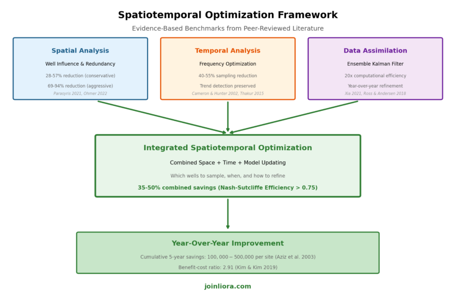
There are three approaches to optimizing a static groundwater monitoring program. You can use spatial and/or temporal analysis to identify redundant wells or wells that contribute little information for decision making. You can also use data assimilation techniques in which you assimilate yearly data into your models to identify opportunities to save money. The figure below outline the pathways towards optimization of a groundwater monitoring network.
Identifying and eliminating redundancy requires systematic analysis that considers both spatial and temporal dimensions of monitoring data. The key insight from this research is that most monitoring networks contain substantial redundancy that traditional design approaches fail to identify. Regulatory requirements typically specify monitoring objectives rather than specific methods, creating flexibility for optimization that many programs fail to exploit.
The economic impact of this redundancy is substantial. A typical 24-well network with quarterly sampling costs approximately 144,000 dollars annually when accounting for mobilization, field labor, analytical testing, and data management. If 35 percent of this monitoring is redundant, the site unnecessarily spends 50,000 dollars each year, compounding to 250,000 dollars over five years. These are resources that could accelerate remediation, support additional characterization, or simply reduce project costs.
Key Takeaway: Spatial optimization achieves 30 to 40 percent well reduction at contaminated sites. Temporal optimization achieves 40 to 55 percent sampling reduction. Combined approaches routinely achieve 35 to 50 percent total savings while maintaining equivalent data quality for decision-making.
Every contaminated site with a monitoring history possesses a valuable asset in its accumulated reports. These documents contain concentration data, hydrogeologic interpretations, and trend analyses that can inform optimization decisions. However, most programs fail to systematically extract and apply the optimization insights embedded in historical data. The result is repeated sampling at wells and frequencies that historical patterns suggest could be reduced without losing meaningful information.
The first step involves compiling concentration time series from all historical reports into a unified database. Many sites possess 10 or more years of quarterly data, representing 40 or more observations per well. This data density exceeds the minimum required for robust statistical analysis and supports sophisticated optimization approaches that were not possible when monitoring began.
Zhou (1996)(3) established that six quarterly observations represent the minimum for trend detection, while longer records enable more sophisticated optimization approaches (https://doi.org/10.1016/0022-1694(95)02892-7). Sites with two or more years of consistent monitoring history possess the data foundation necessary for meaningful optimization analysis. The challenge lies not in data availability but in systematically extracting actionable insights from accumulated records.
Several analytical methods enable extraction of optimization insights from historical data. Trend analysis identifies wells where concentrations have stabilized or achieved regulatory targets, suggesting reduced monitoring frequency may be appropriate. Correlation analysis identifies wells with similar concentration patterns, suggesting spatial redundancy that network reduction could address. Variability analysis identifies wells where concentration fluctuations provide limited additional information beyond what adjacent wells provide.
Liu and colleagues (2012)(4) established a Value of Information framework quantifying the economic worth of monitoring data for remediation decisions at contaminated sites. Their research demonstrated that characterization and remediation costs must be optimized together, and that traditional variance measures inadequately depict economic significance (https://doi.org/10.1007/s11269-011-9970-3). This framework provides a quantitative basis for integrating professional judgment about decision value with statistical measures of information content.
The integration process involves reviewing statistical rankings against professional understanding of site conditions. Wells flagged for removal based on redundancy analysis may have strategic importance that justifies retention. Wells retained by statistical analysis may face access limitations or other practical constraints. The final optimization plan reflects both statistical evidence and professional judgment about site-specific factors.
Key Takeaway: Historical data compilation is the foundation for optimization. Sites with 6 or more quarterly observations per well possess sufficient data for reliable analysis. The challenge is systematic extraction of optimization insights, not data availability.
Well influence analysis quantifies how much each monitoring well contributes to overall network accuracy. Wells with high influence provide information that cannot be obtained from other locations. Wells with low influence provide redundant information that nearby wells already supply. Identifying and ranking wells by influence enables systematic network reduction focused on removing the least influential locations first while preserving the information content essential for site management decisions.
Jones and colleagues (2022)(5) documented the well influence analysis methodology implemented in GWSDAT for contaminated site assessment. The approach compares estimated plume dynamics including mass, area, and concentration between complete datasets and datasets with individual wells removed. Wells whose removal has minimal impact on estimated plume dynamics rank as candidates for reduced sampling or elimination (https://doi.org/10.1111/gwmr.12522). The method provides ordered omission lists achieving 73 to 77 percent validation accuracy in case study applications.
The GWSDAT approach ranks wells from least to most influential, enabling systematic network reduction while monitoring the impact on estimated plume dynamics. Sites can progressively remove wells from the bottom of the influence ranking while tracking changes in plume mass estimates, concentration gradients, and spatial coverage. When removal begins to substantially affect key metrics, the minimum necessary network has been identified.
Professional judgment remains essential when interpreting influence rankings. A well may rank low in influence because it consistently shows non-detect values, but if that well guards a potential migration pathway toward a sensitive receptor, it may warrant retention despite low statistical contribution. Similarly, wells with access challenges or declining condition may warrant removal even if influence rankings suggest moderate contribution. The combination of quantitative analysis and site-specific knowledge produces defensible optimization decisions.
Genetic algorithms provide powerful optimization capability for monitoring network design when more sophisticated analysis is warranted. Reed and colleagues (2000)(6) applied genetic algorithms to minimize monitoring costs while maintaining detection probability at specified levels at contaminated sites (https://doi.org/10.1029/2000WR900232). These evolutionary approaches explore large solution spaces efficiently by combining elements of successful configurations and introducing random variations to identify globally optimal solutions.
Luo and colleagues (2016)(7) developed a probabilistic Pareto genetic algorithm minimizing total sampling costs, mass estimation error, and first and second moment estimation errors simultaneously for contamination monitoring. Monte Carlo analysis demonstrated 35 percent cost savings potential while achieving Pareto-optimal solutions with low variability and high reliability (https://doi.org/ 10.1016/j.jhydrol.2016.01.009 ). The multi-objective formulation enables explicit tradeoff analysis between competing monitoring objectives.
Key Takeaway: Start with GWSDAT's free well influence analysis to rank wells by contribution. Wells with minimal impact on plume characterization are candidates for removal. Never remove wells near active source areas or compliance boundaries without careful analysis.
Sampling frequency decisions should reflect the information content of additional observations relative to their cost. Wells with stable concentrations provide diminishing marginal information as sampling frequency increases. Wells with rapidly changing concentrations may require higher frequency to capture dynamics relevant to management decisions. The optimal frequency balances information value against sampling cost for each well individually rather than applying uniform frequency across the entire network.
Cameron and Hunter (2002)(2) developed the Cost-Effective Sampling methodology achieving 40 percent initial reduction in annual samples, reaching 55 percent with continued optimization at contaminated sites. Their research established that minimum 6 quarterly results per well are required for reliable frequency optimization analysis. Locations with larger rates of change require more frequent sampling, while stable locations warrant reduced frequency (https://doi.org/10.1002/env.582). This differentiated approach captures more information where it matters while reducing unnecessary sampling at stable locations.
Thakur (2015)(1) applied integrated statistical and geostatistical methods at the Bitterfeld-Wolfen contaminated site. Sen's method for temporal optimization recommended sampling intervals of 238 days at the lower quartile, 317 days at the median, and 401 days at the upper quartile. The analysis found that most wells, 287 of 819, were appropriate for annual rather than quarterly sampling, representing substantial frequency reduction from standard practice (https://doi.org/10.3390/hydrology2030148).
McHugh and colleagues (2016)(8) quantified the relationship between monitoring frequency, monitoring duration, and statistical confidence in attenuation rate estimates at contaminated sites. Their analysis revealed the substantial statistical benefits of increased monitoring intensity. Quarterly sampling requires approximately five years to achieve 50 percent accuracy in attenuation rate estimation. Monthly sampling reduces this to 2.7 years, while continuous monitoring compresses the timeline to less than one year (https://doi.org/10.1111/gwat.12407). This research demonstrates that strategic investment in higher-frequency monitoring at key locations can accelerate site closure timelines.
The practical implementation of frequency optimization involves categorizing wells by concentration trend behavior. Wells showing decreasing trends with consistently declining concentrations may warrant reduced frequency once attenuation is established. Wells with stable trends at or near regulatory targets may require only confirmation sampling. Only wells with increasing trends or active concentration dynamics warrant intensive monitoring. This differentiated approach allocates monitoring resources where they generate the most decision-relevant information.
Key Takeaway: Stable wells often require only annual sampling. Use trend analysis to identify wells where reduced frequency maintains statistical validity. Invest saved resources in higher-frequency monitoring at critical locations where concentration dynamics drive decisions.
Multiple peer-reviewed tools now exist for monitoring network optimization at contaminated sites. Each offers distinct strengths and appropriate applications. Understanding these distinctions enables selection of the most appropriate approach for specific site conditions and organizational capabilities. The following comparison focuses on tools specifically developed and validated for contamination monitoring contexts.

GWSDAT provides an accessible entry point for contaminated site analysis with no cost barrier. Jones and colleagues (2022)(5) documented case study applications demonstrating well influence rankings with 73-77 percent validation accuracy (https://doi.org/10.1111/gwmr.12522). Evers and colleagues (2015)(9) described the underlying statistical methodology (https://doi.org/10.1002/env.2347). The tool excels for initial screening and visualization but cannot predict future conditions or adapt to new data automatically.
MAROS implements EPA-standardized methods for trend analysis and network optimization at contaminated sites. Aziz and colleagues (2003)(10) documented implementation finding 10-year optimization savings of 100,000 to 500,000 dollars for individual contaminated sites (https://doi.org/10.1111/j.1745-6584.2003.tb02605.x). The tool provides defensible documentation for regulatory submittals and is particularly appropriate for sites pursuing monitored natural attenuation demonstrations.
LiORA Trends integrates spatial analysis with physics-based groundwater modeling and ensemble Kalman filter data assimilation for contaminated sites. Ross and Andersen (2018)(11) demonstrated that ensemble Kalman filtering outperformed ordinary kriging for TCE plume characterization at Tooele Army Depot by incorporating information about plume development over time under complex site hydrology (https://doi.org/10.1111/gwat.12786). The platform enables year-over-year refinement as monitoring data accumulate, making it particularly appropriate for sites with active remediation systems or complex hydrogeology where understanding improves significantly over time.
The choice between tools depends on site complexity, budget constraints, and optimization objectives. Sites with straightforward hydrogeology and limited budgets can achieve substantial savings using free tools alone. Complex sites with active remediation or regulatory pressure to demonstrate plume stability may justify investment in predictive platforms that provide continuous optimization and defensible forecasting capability.
Key Takeaway: Start with free tools (GWSDAT, MAROS) for initial analysis to identify obvious optimization opportunities. Consider LiORA when predictive capability, continuous optimization, and integration with numerical modeling matter for long-term site management.
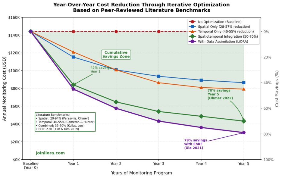
The economic case for monitoring optimization rests on documented savings from peer-reviewed implementations at contaminated sites. Aziz and colleagues (2003)(10) found that 10-year optimization savings typically range from 100,000 to 500,000 dollars for individual contaminated sites. Per-sample costs average 200 to 800 dollars for direct costs including laboratory analysis, field labor, and equipment. When full overhead costs are included, total per-sample costs often exceed 1,000 dollars (https://doi.org/10.1111/j.1745-6584.2003.tb02605.x). Below is an example of how savings accumulate for groundwater monitoring networks based on literature work.
Consider a typical 24-well network with quarterly sampling at 1,500 dollars per sample event including mobilization, sampling, and laboratory analysis. Annual baseline cost is 144,000 dollars. Conservative 35 percent optimization yields 50,400 dollars annual savings. Over five years, cumulative savings exceed 250,000 dollars even without accounting for additional optimization in subsequent years. These savings represent resources available for other environmental management priorities or direct return to organizational budgets.
Optimization analysis typically costs 15,000 to 30,000 dollars for initial assessment depending on network complexity and data availability. Projects achieving 35 percent savings pay back analysis costs within the first year of implementation through reduced monitoring expenses. Subsequent years deliver pure savings with minimal additional analysis investment as the optimization framework becomes established.
The economic benefits extend beyond direct cost reduction. Optimized monitoring programs generate cleaner datasets by eliminating redundant measurements that add noise to statistical analyses. Clearer concentration trends support more defensible regulatory decisions and can accelerate site closure timelines. The combination of cost reduction and improved decision support creates value that substantially exceeds the direct monitoring savings.
Typical ROI Timeline for Monitoring Optimization:
Key Takeaway: Optimization delivers 3:1 to 5:1 return on investment over five years. Initial analysis costs are typically recovered within the first year of implementation. The compounding effect of annual refinement produces savings that substantially exceed initial estimates.
The most effective optimization follows an iterative annual cycle rather than a one-time analysis. Each year's monitoring data informs refinements to the following year's sampling strategy, creating compounding benefits as understanding improves. This approach addresses the reality that optimal monitoring networks evolve as plumes migrate, remediation progresses, and site understanding deepens.
Herrera and Pinder (2005)(12) published foundational research on space-time optimization of groundwater quality sampling networks at contaminated sites. Their approach coupled Kalman filtering with stochastic contaminant transport modeling for simultaneous space-time optimization (https://doi.org/10.1029/2004WR003626). The methodology minimizes estimate error variance while enabling real-time concentration updates, addressing the economic burden of long-term quality monitoring through combined spatial-temporal redundancy analysis.
Kollat, Reed, and Maxwell (2011)(13) introduced the ASSIST framework combining flow-and-transport modeling, bias-aware ensemble Kalman filtering, and many-objective evolutionary optimization for contaminated groundwater monitoring. The framework accounts for systematic model errors while forecasting value of new observation investments across multiple objectives simultaneously (https://doi.org/10.1029/2010WR009194). This represents the most sophisticated integration of spatial and temporal optimization available in the peer-reviewed literature for contamination applications.
Documentation of year-over-year improvement requires consistent metrics tracked from baseline through each optimization cycle. Recommended metrics include total annual monitoring cost, number of wells sampled, average sampling frequency, plume mass estimate uncertainty, and regulatory compliance status. Trend analysis of these metrics over multiple years demonstrates progressive improvement and builds confidence for continued optimization. Clear documentation also supports knowledge transfer when project personnel change.
Key Takeaway: Optimization is not a one-time event. Annual review cycles compound savings over time while maintaining regulatory defensibility through continuous documentation of outcomes.
Zhou (1996)(3) established that six quarterly observations represent the minimum for reliable trend detection at each well. Most sites with two or more years of monitoring history possess sufficient data for initial optimization analysis. Longer records enable more sophisticated approaches and higher confidence in recommendations. Sites with 10 or more years of quarterly data can support advanced spatiotemporal analysis methods that reveal seasonal patterns and long-term trends not visible in shorter records.
Regulators typically specify monitoring objectives rather than specific methods or frequencies. Optimization proposals supported by peer-reviewed methods and documented in tools like GWSDAT or MAROS generally receive acceptance when they demonstrate equivalent information content for decision-making. The key is providing clear technical justification showing that reduced monitoring maintains the ability to detect changes relevant to regulatory compliance and remediation performance. Building regulatory relationships and presenting optimization proposals proactively rather than reactively increases acceptance likelihood.
Kollat and colleagues (2011)(13) maintained Nash-Sutcliffe efficiency above 0.75 in their many-objective optimization framework. Most practitioners accept 5-10 percent reduction in mapping accuracy in exchange for 30-50 percent cost savings, provided detection capability for concentration changes relevant to decisions remains intact. The acceptable threshold depends on regulatory context and consequences of missed detections at each specific site.
Start with wells that rank lowest in influence analysis AND show stable concentration trends AND face accessibility challenges. This combination identifies wells where removal risk is lowest and practical benefits are highest. Never remove wells near active source areas, compliance boundaries, or downgradient receptor locations without careful analysis demonstrating that remaining wells provide adequate coverage for detecting migration toward sensitive locations. Consider seasonal access issues and sampling efficiency when evaluating candidates.
Yes, but with appropriate caution regarding locations where concentration dynamics drive remediation decisions. Ross and Andersen (2018)(11) demonstrated ensemble Kalman filter optimization during active TCE remediation at Tooele Army Depot-North. The key is ensuring optimization maintains ability to detect concentration changes relevant to remediation performance assessment and system operation decisions. Wells monitoring extraction system capture, treatment performance, or injection effects generally warrant retention regardless of influence rankings.
Networks with fewer than 10 wells offer limited optimization potential because baseline redundancy is typically low in sparse networks. Networks with 20 or more wells consistently demonstrate substantial redundancy amenable to systematic reduction. The greatest savings potential exists at sites with 30 or more wells installed over time without systematic design optimization, often representing decades of incremental network expansion in response to changing regulatory requirements or expanding contamination boundaries.
Documentation should include baseline network description, analysis methodology, well rankings with supporting statistics, proposed modifications, and projected cost savings. Tools like GWSDAT and MAROS generate standardized reports suitable for regulatory submittal. Include comparison of plume characterization metrics before and after optimization to demonstrate maintained data quality. Reference peer-reviewed literature to establish defensibility of methods employed.
1. J. Thakur, Optimizing Groundwater Monitoring Networks Using Integrated Statistical and Geostatistical Approaches. HYDROLOGY 2, 148-175 (2015).
2. K. Cameron, P. Hunter, Using spatial models and kriging techniques to optimize long-term ground-water monitoring networks: a case study. ENVIRONMETRICS 13, 629-656 (2002).
3. Y. Zhou, Sampling frequency for monitoring the actual state of groundwater systems. JOURNAL OF HYDROLOGY 180, 301-318 (1996).
4. X. Liu, J. Lee, P. Kitanidis, J. Parker, U. Kim, Value of Information as a Context-Specific Measure of Uncertainty in Groundwater Remediation. WATER RESOURCES MANAGEMENT 26, 1513-1535 (2012).
5. W. Jones, L. Rock, A. Wesch, E. Marzusch, M. Low, Groundwater Spatiotemporal Data Analysis Tool: Case Studies, New Features and Future Developments. GROUND WATER MONITORING AND REMEDIATION 42, 14-22 (2022).
6. P. Reed, B. Minsker, A. Valocchi, Cost-effective long-term groundwater monitoring design using a genetic algorithm and global mass interpolation. WATER RESOURCES RESEARCH 36, 3731-3741 (2000).
7. Q. Luo, J. Wu, Y. Yang, J. Qian, J. Wu, Multi-objective optimization of long-term groundwater monitoring network design using a probabilistic Pareto genetic algorithm under uncertainty. JOURNAL OF HYDROLOGY 534, 352-363 (2016).
8. T. McHugh, P. Kulkarni, C. Newell, Time vs. Money: A Quantitative Evaluation of Monitoring Frequency vs. Monitoring Duration. GROUNDWATER 54, 692-698 (2016).
9. L. Evers, D. Molinari, A. Bowman, W. Jones, M. Spence, Efficient and automatic methods for flexible regression on spatiotemporal data, with applications to groundwater monitoring. ENVIRONMETRICS 26, 431-441 (2015).
10. J. Aziz, M. Ling, H. Rifai, C. Newell, J. Gonzales, MAROS: A decision support system for optimizing monitoring plans. GROUND WATER 41, 355-367 (2003).
11. J. Ross, P. Andersen, The Ensemble Kalman Filter for Groundwater Plume Characterization: A Case Study. GROUNDWATER 56, 571-579 (2018).
12. G. Herrera, G. Pinder, Space-time optimization of groundwater quality sampling networks - art. no. W12407. WATER RESOURCES RESEARCH 41, (2005).
13. J. Kollat, P. Reed, R. Maxwell, Many-objective groundwater monitoring network design using bias-aware ensemble Kalman filtering, evolutionary optimization, and visual analytics. WATER RESOURCES RESEARCH 47, (2011).
For integrated monitoring optimization with predictive capability and continuous refinement at contaminated sites, contact us.
