I spend considerable time thinking about how we measure things underground. The physical act of lowering a bailer into a well or watching a pump purge three volumes of stagnant water forms only part of the story. The deeper question concerns what those groundwater measurements tell us and what the measurements fail to reveal.
Peer-reviewed literature on this subject reveals something that should concern anyone managing a contaminated site: the frequency with which we collect groundwater samples determines what we can know about our plumes.
This determination operates through mathematics that permit no negotiation:
The difference between these approaches is not incremental but represents a fundamental divide in the quality and type of information available for decision-making. In other words, high frequency data is not merely different in magnitude but different in type from point in time estimates of groundwater concentrations.
Quarterly sampling programs generate four data points per year from each monitoring location. These four points must support:
The mathematics of statistical inference place bounds on what four annual observations can accomplish regardless of analytical precision or sampler technique.
Consider trend detection as an example. Demonstrating that concentrations are declining requires sufficient data to establish statistical significance against a backdrop of natural variability. Groundwater concentrations fluctuate in response to recharge events, seasonal patterns, and stochastic processes.
The fluctuations are termed variance and are a natural component of an ecosystem. The foundation of a statistical test is the analysis of this variance. In machine learning terms, this variance can be thought of as aleatoric uncertainty:
Epistemic uncertainty is the uncertainty about the model due to finite training data and an imperfect learning algorithm. Aleatoric uncertainty is due to the inherent irreducible randomness in a process from the perspective of a model. Alet et al. 2025(1) (https://doi.org/10.48550/arXiv.2506.10772)
Four observations per year cannot distinguish signal from noise when variability approaches or exceeds the underlying trend. The result is uncertainty that persists for years while sparse data accumulate.
The peer-reviewed literature quantifies these limitations. McHugh, Kulkarni, and Newell established in Groundwater(2) that five years of quarterly sampling provide the minimum data density to establish attenuation rates with acceptable statistical confidence under typical site conditions.
This timeline means that sites requiring trend demonstration cannot achieve that goal in less than five years regardless of how fast concentrations decline. The limitation arises from information content, not from site conditions or regulatory requirements.
Two papers fundamentally shape my thinking on groundwater monitoring frequency:
Paper 1: Papapetridis and Paleologos in Water Resources Management(3) examines how sampling frequency affects contamination detection
Paper 2: McHugh and colleagues in Groundwater(2) addresses how monitoring frequency influences attenuation rate characterization
Together, these works build a case that traditional quarterly sampling programs cannot support the decisions we ask them to inform.
Both papers employ mathematical frameworks that yield conclusions independent of site-specific conditions. The relationships they identify between monitoring frequency and outcome metrics apply across hydrogeologic settings and contaminant types.
Autonomous groundwater sensors capable of continuous measurement represent the technological development that transforms these findings from academic observations to actionable insights. The ability to generate thousands of data points per year per monitoring location changes the fundamental calculus of detection and characterization.
Papapetridis and Paleologos approached groundwater monitoring from a probabilistic perspective in their 2012 Water Resources Management study (https://doi.org/10.1007/s11269-012-0039-8). Using Monte Carlo simulations of contaminant transport through heterogeneous aquifers, they asked a straightforward question: given a monitoring network of a certain size, sampled at a certain frequency, what is the probability of detecting a contamination event?
The answers they obtained should concern anyone relying on quarterly monitoring for release detection.
Their simulations revealed that a network of eight monitoring wells, even when sampled daily, achieves a maximum detection probability of only 50 percent under optimal conditions. Put differently, half of all contamination events would remain undetected.
To achieve detection probabilities that exceed failure probabilities across a range of hydrogeologic conditions, they found that 20 wells sampled monthly were required. The mathematics here permits no negotiation: detection probability decreases as monitoring frequency decreases.
In highly dispersive subsurface environments, this relationship becomes especially pronounced. Dispersion spreads contaminants across wider areas more quickly, meaning that the temporal window during which contamination might be observed at any single monitoring location narrows.
Less frequent sampling increases the probability that contamination will pass through the monitoring network between sampling events, yielding false assurance of site stability.
The Papapetridis and Paleologos work introduced a concept they termed remedial action delay. This concept recognizes that contamination detection is not an end in itself. Between the moment contaminants first arrive at monitoring locations and the moment they appear in collected samples, time passes. During that time, plumes continue to spread.
In highly dispersive environments with infrequent sampling, the observed delay between contamination arrival and detection can extend to years. The plume expansion that occurs during this delay increases remediation scope and costs in proportion to the delay duration.
The 2012 study quantified this relationship through systematic variation of monitoring frequency in Monte Carlo simulations. For quarterly sampling programs:
These findings apply to sites relying on quarterly monitoring for release detection. The delayed detection translates to larger cleanup obligations and extended project timelines.
A natural question arises: can increased network density compensate for reduced sampling frequency? Can we deploy more monitoring wells sampled less frequently and achieve equivalent detection performance?
The Papapetridis and Paleologos analysis suggests the answer is no for practical network sizes. Even substantially increasing well counts cannot overcome the fundamental limitation that contamination events occurring between sampling intervals remain invisible until the next sample collection.
The interaction between spatial coverage and temporal resolution creates dependencies that prevent simple tradeoffs. Detection requires both adequate spatial coverage and adequate temporal resolution.
Detection represents only the first challenge that monitoring frequency determines. Once contamination is known to exist, site managers must characterize how concentrations change over time. This characterization supports critical decisions:
All three questions require trend analysis with sufficient statistical power to distinguish real changes from measurement noise and natural variability.
McHugh, Kulkarni, and Newell published their seminal analysis "Time vs. Money" in Groundwater(2) in 2016 (https://doi.org/10.1111/gwat.12407). The paper examined a question that should concern every site manager: what is the optimal balance between monitoring frequency and monitoring duration?
Their analysis revealed something counterintuitive. Most site managers assume that more frequent sampling accelerates trend demonstration. The McHugh analysis confirmed this intuition but quantified the relationship in ways that challenge conventional monitoring programs.
Under typical site conditions with quarterly sampling, achieving statistical confidence in concentration trends requires a minimum of five years of data. This duration reflects the interaction between:
Five years represents the minimum under favorable conditions. Sites with high variability or subtle trends require longer periods.
The McHugh analysis demonstrated that increasing sampling frequency can reduce the time required to achieve statistical confidence. Monthly sampling can reduce the required monitoring period to 3 to 4 years. Weekly sampling can further reduce this to 2 to 3 years.
However, traditional field sampling and laboratory analysis make high-frequency monitoring economically prohibitive. The cost of monthly sampling exceeds quarterly sampling by a factor of three. Weekly sampling costs twelve times as much as quarterly programs.
This economic constraint has locked most sites into quarterly sampling programs despite the knowledge that more frequent monitoring would accelerate trend characterization.
Autonomous sensors that measure continuously at costs competitive with quarterly sampling eliminate this constraint. When sensors cost the same as or less than quarterly sampling while providing measurements every 30 minutes, the frequency-duration tradeoff shifts decisively in favor of continuous monitoring.
The McHugh framework provides the mathematical basis for understanding this shift. Their analysis shows that measurement frequency has the strongest influence on time to statistical confidence, stronger than the total number of measurements or the monitoring duration.
Continuous monitoring provides measurement frequencies 4,380 times higher than quarterly sampling, fundamentally altering what can be achieved within practical project timelines.
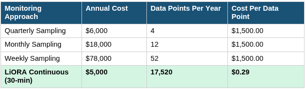
Table 1 reveals the fundamental economics of monitoring frequency decisions. Traditional sampling incurs a fixed cost of approximately $1,500 per event regardless of frequency. This cost includes mobilization, purging, sample collection, chain of custody, laboratory analysis, and data management. Increasing frequency through traditional methods therefore increases costs linearly. Continuous sensor monitoring breaks this relationship by generating thousands of measurements for a single annual fee. The cost per data point drops by more than 99 percent compared to traditional sampling.
Traditional groundwater monitoring evolved in an era when every sample required:
These costs made quarterly sampling the economic equilibrium between inadequate monitoring and budget exhaustion. Most sites settled on quarterly frequency not because it optimally serves site objectives but because it represents affordable inadequacy.
Some sites with higher budgets or greater contamination concerns implement monthly monitoring. This approach improves detection probability and accelerates trend characterization compared to quarterly programs. However, monthly monitoring costs three times as much as quarterly sampling while still providing only 12 data points per year.
The improvement is real but remains constrained by sparse temporal resolution that prevents detection of:
Continuous monitoring with autonomous sensors measures every 30 minutes, generating 17,520 data points per year from each monitoring location. This frequency enables:
Detection advantages:
Characterization advantages:
Cost advantages:
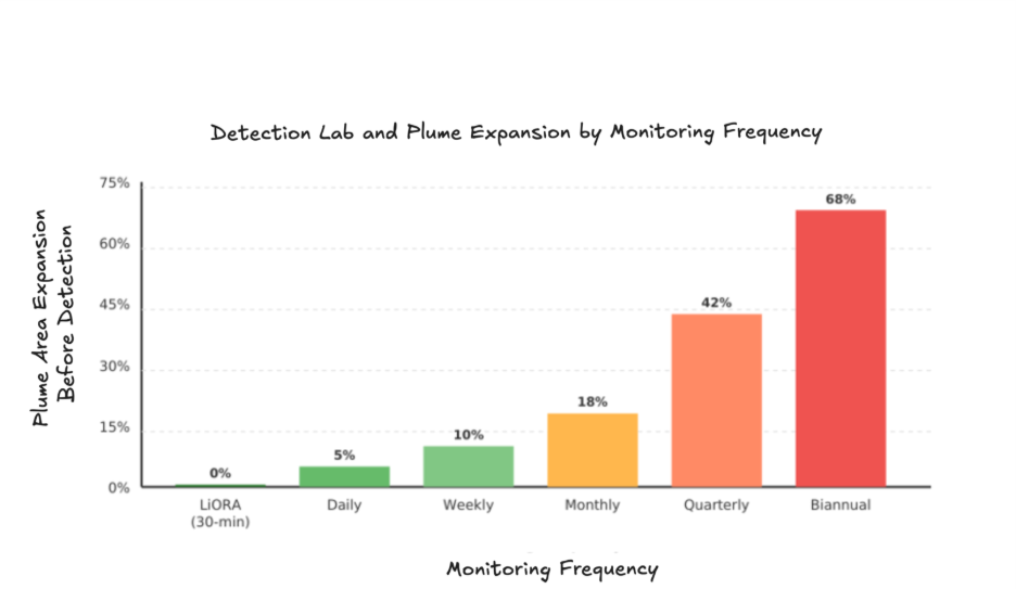
Figure 1 presents the relationship between monitoring frequency and plume area expansion before detection based on peer-reviewed simulation results. The data demonstrate that quarterly sampling, the industry standard, allows plumes to expand by more than 40 percent before observation. Biannual sampling approaches 70 percent expansion. Continuous monitoring through LiORA sensors reduces expansion to near zero by eliminating detection lag entirely.
Most site managers underestimate the full cost of quarterly monitoring by focusing only on laboratory fees. A complete accounting of quarterly sampling costs reveals expenses that exceed $6,000 per well per year:
Field Activities (40-50% of total):
Laboratory Analysis (25-35% of total):
Data Management (20-30% of total):
Annual total: $5,400 to $7,200 per well depending on contaminant parameters and site access.
LiORA continuous monitoring costs $5,000 per sensor per year, a single figure that covers:
This represents 17% cost savings compared to quarterly sampling while providing 4,380 times more data.
The break-even analysis for continuous monitoring versus traditional sampling depends on site-specific factors:
Direct Cost Comparison:
For a 10-well monitoring network:
Value Beyond Direct Cost Savings:
The break-even calculation based solely on monitoring costs understates the true economic advantage because it ignores:
A comprehensive ROI analysis includes three components:
Component 1: Direct Monitoring Cost Savings
Component 2: Accelerated Project Completion
Component 3: Improved Outcomes
Total 10-year ROI: $600,000 for a typical mid-sized site
Payback period: Less than 1 year in most scenarios when all value components are included.
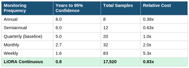
Table 2 presents the time required to achieve statistical confidence in attenuation rate estimates under different monitoring approaches. The data derive from the mathematical relationships established by McHugh and colleagues. Quarterly sampling requires five years to achieve 95 percent confidence. LiORA continuous monitoring achieves the same confidence in less than one year while costing 17 percent less than quarterly sampling. This represents an 84 percent reduction in time to regulatory milestone achievement.
Autonomous groundwater sensors deploy directly in monitoring wells where they measure contaminant concentrations continuously without human intervention. The sensors remain in place for years, measuring every 30 minutes and transmitting data wirelessly to cloud-based analysis platforms.
Modern sensor technology has overcome the limitations that previously prevented widespread adoption:
Power Management:
Measurement Accuracy:
Data Transmission:
Deployment Simplicity:
The temporal resolution of continuous monitoring reveals patterns invisible to quarterly sampling:
Seasonal Variations:
Episodic Events:
Temporal Trends:
Spatial Patterns:
Continuous monitoring integrates with traditional sampling programs through several approaches:
Parallel Monitoring:
Hybrid Programs:
Complete Replacement:
What LiORA Sensors Measure:
How LiORA Sensors Work:
LiORA Sensor Advantages:
Platform Capabilities:
Integration With Existing Tools:
User Interface:
LiORA Sensor Pricing:
LiORA Trends Pricing:
Cost Comparison:
Value Delivered:
Step 1: Site Assessment (Week 1)
Step 2: Pilot Deployment (Weeks 2-4)
Step 3: Full Implementation (Weeks 5-8)
Step 4: Optimization (Ongoing)
Pre-Deployment Consultation:
During Implementation:
Ongoing Compliance:
Detection Performance:
Characterization Performance:
Economic Performance:
Regulatory Performance:
Optimal monitoring frequency depends on site objectives. For release detection, peer-reviewed research by Papapetridis and Paleologos(3) indicates that monthly sampling represents the minimum frequency to prevent substantial plume expansion during detection delays.
For trend characterization, McHugh and colleagues(2) demonstrated that quarterly sampling requires 5+ years to achieve statistical confidence, while higher frequency accelerates this timeline. Continuous monitoring satisfies both objectives simultaneously by providing the high temporal resolution needed for detection while generating the data density needed for statistical analysis.
Traditional quarterly sampling costs approximately $6,000 per well per year when all costs are properly accounted, including mobilization ($600-$1,200/year), purging and sampling labor ($800-$1,600/year), laboratory analysis ($600-$1,600/year), and data management ($600-$1,200/year).
LiORA Sensors cost $5,000 per sensor per year, covering continuous measurement every 30 minutes, wireless data transmission, automated quality assurance, platform access, and technical support. This represents 17% cost savings while providing 4,380 times more data.
Continuous monitoring provides 17,520 data points per year compared to 4 from quarterly sampling, enabling:
Detection advantages: Contamination events visible within 30 minutes instead of up to 90 days, eliminating detection delays that allow 200-400% plume expansion
Characterization advantages: Statistical confidence achieved in less than 1 year instead of 5+ years required with quarterly sampling
Cost advantages: $5,000 per sensor per year vs $6,000 per well for quarterly sampling
Decision-making advantages: Real-time data enables immediate response to changing conditions rather than discovering problems months after they occur
Yes, in many cases. Continuous monitoring provides superior detection and characterization performance compared to quarterly sampling at lower cost. However, regulatory requirements vary by jurisdiction. Some programs require periodic laboratory confirmation even when continuous sensors provide primary monitoring data.
LiORA works with clients to design monitoring programs that meet regulatory requirements while maximizing the benefits of continuous data. Many sites use continuous monitoring as the primary program with annual or semiannual laboratory confirmation sampling.
LiORA sensors measure petroleum hydrocarbon concentrations with accuracy comparable to laboratory analysis. The sensors undergo calibration against certified reference standards and include quality assurance protocols that flag questionable measurements for review.
Continuous measurement captures temporal variability that discrete sampling misses, providing a more complete picture of actual site conditions than the four annual snapshots from quarterly sampling. The 17,520 annual measurements per sensor enable statistical characterization of measurement uncertainty.
LiORA sensors measure petroleum hydrocarbon concentrations directly. This includes:
The sensors provide the contaminant-specific data needed for regulatory compliance and transport modeling. Contact LiORA Technologies to discuss sensor capabilities for specific contaminants of concern at your site.
Sensor installation typically requires 1 to 2 days depending on monitoring network size. The sensors fit standard monitoring well diameters (2 inches and larger) and deploy using conventional wireline equipment. No modifications to well construction are required.
Sites can begin generating continuous data within days of installation. The rapid deployment timeline allows sites to begin realizing the benefits of continuous monitoring without extended project development periods.
LiORA sensors operate continuously for 2+ years on battery power before requiring battery replacement or sensor retrieval. The long deployment duration minimizes maintenance requirements and ensures uninterrupted data collection.
When sensors require service, replacement sensors can be deployed quickly to maintain continuous monitoring. LiORA provides deployment and retrieval services or can train site personnel for self-service deployments.
Continuous monitoring data is increasingly accepted by regulatory agencies as the technology matures and case studies demonstrate reliability for compliance applications. USGS guidelines now recognize that high-frequency monitoring provides capabilities that traditional sampling cannot match.
LiORA works with clients to ensure data formats, quality assurance protocols, and reporting structures meet the specific requirements of relevant regulatory programs. Early engagement with regulators during program design helps ensure acceptance for intended applications.
Yes. Site closure requires demonstrating plume stability and concentration trends with statistical confidence. Continuous monitoring achieves the statistical confidence required for closure demonstrations in less than one year rather than the five or more years required with quarterly sampling.
Many sites find that continuous monitoring data provide the statistical power needed to support closure applications that seemed unattainable with sparse quarterly data. The enhanced temporal resolution also enables demonstration of seasonal stability that quarterly sampling cannot document.
Continuous monitoring supplements rather than replaces compliance sampling where regulatory programs specify discrete sampling requirements. However, continuous monitoring data often support requests for reduced sampling frequency under regulatory flexibility provisions.
Demonstrating plume stability through continuous monitoring can justify transition from quarterly to semiannual or annual compliance sampling. The resulting cost savings often offset the cost of continuous monitoring.
Return on investment depends on site-specific factors including current monitoring costs, regulatory timeline requirements, and liability exposure. Sites typically realize value through three mechanisms:
Direct cost savings: $1,000 per location per year from lower monitoring costs
Accelerated site closure: 4+ years reduction in program duration worth $200,000-$400,000
Improved decision-making: Better remediation optimization and reduced liability worth $100,000-$300,000
Total 10-year ROI typically exceeds $500,000 for a mid-sized site. Payback period is typically less than one year when all value components are included.
The break-even point for continuous monitoring versus traditional sampling is immediate based on direct cost comparison:
When accelerated project completion and improved decision-making are included, the value proposition becomes even more compelling. Sites achieve positive ROI in the first year of deployment through combination of:
Contact LiORA Technologies to schedule a site assessment:
The assessment evaluates:
The LiORA team develops:
Implementation can begin within weeks of engagement for sites ready to advance to continuous monitoring.
Contact LiORA to learn how continuous monitoring can accelerate your site closure timeline by 84% while reducing monitoring costs by 17%.

As CEO of LiORA, Dr. Steven Siciliano brings his experience as one of the world’s foremost soil scientists to the task of helping clients to efficiently achieve their remediation goals. Dr. Siciliano is passionate about developing and applying enhanced instrumentation for continuous site monitoring and systems that turn that data into actionable decisions for clients.